5.1 Describing one variable

5.1.1 Summary statistics

A useful first step in analyzing the distribution of scores on a single numeric variable is to calculate the relevant summary statistics. Use the summary() function for a quick, general overview. This returns the minimum, mean, and maximum scores, as well as the score at 1st, 2nd (median), and 3rd quartiles.

  summary(dcps)  # for every variable in the data frame

##     SchCode      SchName                SchType  
##  Min.   :202   Length:108         Elementary:64  
##  1st Qu.:264   Class :character   Middle    :25  
##  Median :318   Mode  :character   High      :19  
##  Mean   :340                                     
##  3rd Qu.:414                                     
##  Max.   :943                                     
##    NumTested       ProfLang       ProfMath    
##  Min.   :  12   Min.   : 0.0   Min.   : 0.00  
##  1st Qu.: 112   1st Qu.:12.3   1st Qu.: 9.38  
##  Median : 146   Median :19.1   Median :20.56  
##  Mean   : 180   Mean   :29.7   Mean   :26.96  
##  3rd Qu.: 212   3rd Qu.:40.0   3rd Qu.:36.88  
##  Max.   :1423   Max.   :94.1   Max.   :82.76  
##  DataVERSION       
##  Length:108        
##  Class :character  
##  Mode  :character  
##                    
##                    
## 

  summary(dcps$ProfLang) # for a specific variable

##    Min. 1st Qu.  Median    Mean 3rd Qu.    Max. 
##     0.0    12.3    19.1    29.7    40.0    94.1

For specific inquiries, use the summarize() function and customize your report. For example:

  dcps %>%   # start by piping in the dataset
    summarize(
      Avg = mean(ProfLang), # calculates the mean
      StdDev = sd(ProfLang),   # standard deviation
      Range = max(ProfLang) - min(ProfLang) 
    )

## # A tibble: 1 x 3
##     Avg StdDev Range
##   <dbl>  <dbl> <dbl>
## 1  29.7   24.6  94.1

5.1.2 Graphing the distribution

We typically use a histogram or box plot to visualize the distribution of scores on a numeric variable.

# Basic histogram
  hist(dcps$ProfLang)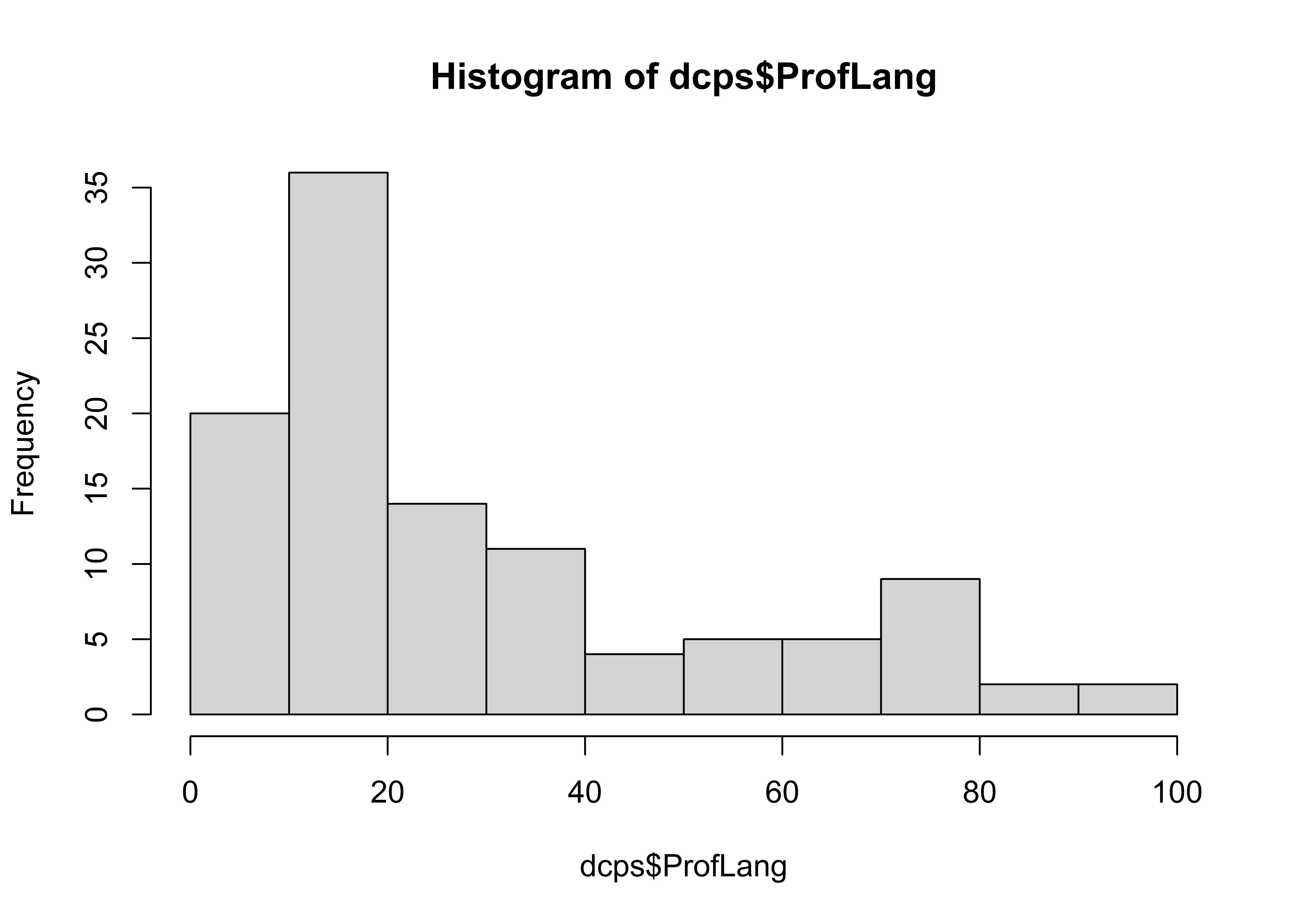

# Basic boxplot
  boxplot(dcps$ProfLang, horizontal = TRUE)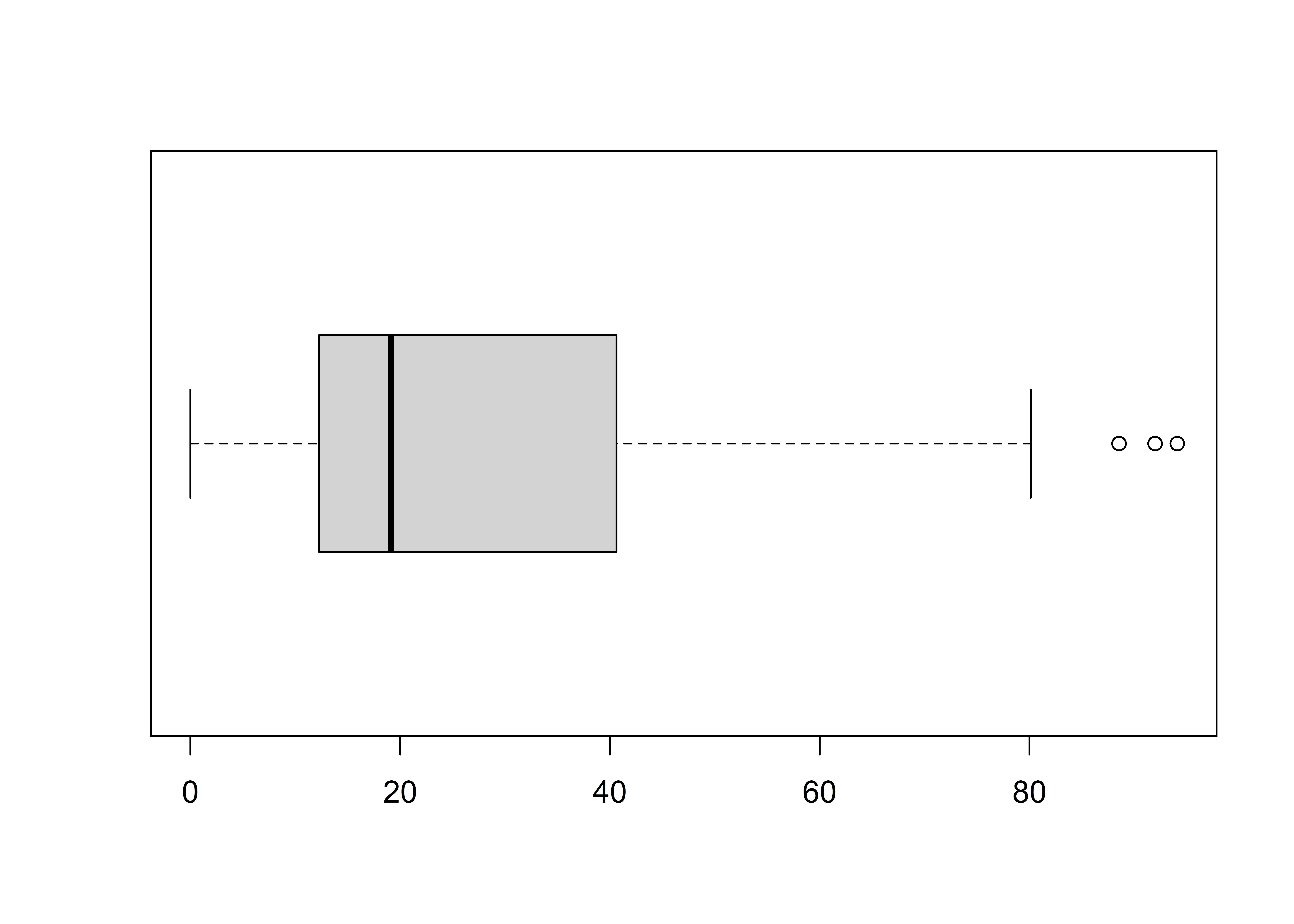

See the chapter on data visualization to learn how to format these graphs appropriately for academic or professional settings.

5.1.3 Testing hypotheses

A one-sample \(t-\)test (t.test()) compares the observed mean on a numeric variable to a hypothesized mean. The resulting \(p\)-value indicates the probability of observing the mean in your data from a population defined by the null hypothesis (mu =).

For example, evaluate the argument that at least half of DC public school pupils read at or above grade level (i.e. \(H_0:~\mu \geq 50\)).

  t.test(dcps$ProfLang, mu = 50, alternative = 'less')

## 
##  One Sample t-test
## 
## data:  dcps$ProfLang
## t = -8.6, df = 107, p-value = 5e-14
## alternative hypothesis: true mean is less than 50
## 95 percent confidence interval:
##   -Inf 33.66
## sample estimates:
## mean of x 
##     29.73

The test results suggest that it is extremely unlikely (\(t=-8.6\), \(p<0.001\)) that we would observe these data if the majority of DC public school pupils read at or above grade level. We can reject the null hypothesis.